A MODEL FOR THE EVOLUTION OF NUCLEOTIDE POLYMERASE
DIRECTIONALITY
by
Joshua Ballanco
A DISSERTATION
Submitted to the Faculty of the Stevens Institute of Technology
in partial fulfillment of the requirements for the degree of
DOCTOR OF PHILOSOPHY
STEVENS INSTITUTE OF TECHNOLOGY
Castle Point on Hudson
Hoboken, NJ 07030
2011
© 2011, Joshua Ballanco. All rights reserved.
A MODEL FOR THE EVOLUTION OF NUCLEOTIDE POLYMERASE
DIRECTIONALITY
ABSTRACT
In all known living organisms, every enzyme that synthesizes nucleic acid polymers does so by adding nucleotide 5’-triphosphates to the 3’-hydroxyl group of the growing chain. This results in the well known 5′→ 3′ directionality of all DNA and RNA Polymerases. The lack of any alternative mechanism, e.g. addition in a 3′→ 5′ direction, may indicate a very early founder effect in the evolution of life, or it may be the result of a selective pressure against such an alternative. In an attempt to determine whether the lack of an alternative polymerase directionality is the result of a founder effect or evolutionary selection, we have constructed a basic model of early polymerase evolution. This model is informed by the essential chemical properties of the nucleotide polymerization reaction. With this model, we are able to simulate the growth of organisms with polymerases that synthesize either 5′→ 3′ or 3′→ 5′ in isolation or in competition with each other. We have found that a competition between organisms with 5′→ 3′ polymerases and 3′→ 5′ polymerases only results in a evolutionarily stable strategy under certain conditions. Furthermore, we have found that mutations lead to a much clearer delineation between conditions that lead to a stable coexistence of these populations and conditions which ultimately lead to success for the 5′→ 3′ form. In addition to presenting a plausible explanation for the uniqueness of enzymatic polymerization reactions, we hope these results also provide an example of how whole organism evolution can be understood based on molecular details.
Author: Joshua Ballanco
Advisor: Marc Mansfield
Date: May 9th, 2011
Department: Chemistry, Chemical Biology, and Biomedical Engineering
Degree: Doctor of Philosophy
Dedication
This thesis is dedicated to my loving and supportive wife Ceren
Acknowledgements
I would like to acknowledge Marc Mansfield for the years of guidance, inspiration, and instruction that he so graciously provided during both my undergraduate and graduate education. I would also like to acknowledge Francis Jones for making this research possible, for the encouragement that he provided me as an undergraduate and the opportunity he made available to me as a graduate. I would also like to thank the members of my committee, Philip Leopold, A. K. Ganguly, Knut Stamnes, and Nicholas Murgolo, for their input and invaluable insight. Thanks also go out to the faculty and staff of the Department of Chemistry, Chemical Biology, and Biomedical Engineering for all the help they have provided through the years, and most especially to Mary Newell without whom I would not have made it past the first day of graduate school. Finally, I must humbly admit that the thesis presented here would not exist if it were not for the constant support and encouragement of my beautiful wife Ceren Örnek-Ballanco.
Evolution has classically been a science of the past. That is, the primary sources of evidence used in the formulation and validation of evolutionary theory have been the fossil record, geology, and observations of the current form and distribution of species as a result of events that took place in the past. Where evolution does exhibit predictive power, it is primarily in the ability to predict what new evidence from the past should eventually be revealed, such as the many fossils of transitional forms discovered over the past centuries. In this regard, evolution has been wildly successful.
Where the study of Evolution has been thus far lacking is in its ability to predict the future. That is, looking at a collection of fossils and historical records of environmental conditions, evolutionary theory gives us the ability to identify which selective pressures acted on past populations. What evolutionary theory cannot do, at present, is predict which environmental conditions or physical forms will act as selective pressures in the future. At best, we can make educated guesses based on past evidence, but we lack the ability to assign a concrete measure of confidence in such predictions. In the end, the only sure way to determine which individuals are best fit is to wait and see which individuals ultimately survive and reproduce.
This is not an inherent failing of evolution, but rather a sign of a young and developing field. The inability to predict the future course of evolution is tied directly to the fact that selective pressures can come from practically any feature of an organism. Everything from diet to behavior to physical form can lead to a selection for or against the eventual reproductive success of an organism. The situation in which evolution finds itself is akin to what physics would be like if every projectile had its own unique laws of motion. What evolution desperately needs is a fundamental set of principles from which the success of any organism can be derived, much as the path of every projectile can ultimately be derived from Newton’s laws of motion.
The implications of a coherent method for deriving the evolutionary success of an individual undergoing natural selection would be far reaching. Perhaps the most obvious implication would be an improved ability to predict patterns of disease emergence and transmission. Cancer treatment would be another potential area of benefit, as cancer is an evolutionary process. With each round of chemotherapy or radiation treatment, those cancer cells which are better adapted to resist treatment will survive. These cells will then seed a reemergent, more difficult to treat, tumor. Understanding the dynamics of evolution, and how to predict the future course of evolution, would improve our ability to design effective treatments for both microbial diseases and cancer.
Even non-biological processes are driven by evolution and obey many of the same laws that Darwin first laid out 150 years ago. Both languages and economies undergo evolutionary processes, driven by the same math as cancer or the origin of species[10]. That said, we must make a distinction between biological and non-biological evolution. The reason for doing so lies in the approaches that can be taken to investigate each type of evolutionary system. We know far more about biological organisms than merely that they evolve. The past 50 years has seen an explosion of knowledge about the chemistry of life and the operation of those molecular systems which compose cells and influence the phenotypes of complex multicellular organisms.
For this reason, biological systems undergoing evolution present a unique opportunity to attempt to derive the fundamental principles of evolution from the individual mechanics of the evolving systems. Specifically, with biology we can explore the feedback mechanism which drives evolution: the “Central Dogma” of biology. This is the pathway by which information flows from an organism’s nucleic acids, where it is stored, to the organism’s proteins which then drive fundamental biochemical processes[14]. These biochemical processes determine the phenotypes eventually selected for or against in the process of natural selection. From this flow of information, it is understood that those organisms which contain the information for generating the better fit traits will become enriched in the population, and therefore will pass on this information in greater numbers than their less fit peers[4].
The biochemical processes that ultimately result in phenotypic traits can be very complex, and their ultimate effect may be indirect. This makes it difficult to study the biochemical evolution of all but the simplest of traits in the simplest of organisms. One biochemical process that is relatively simple, and whose impact has a very direct effect on the eventual transmission of genetic information, is the process of nucleotide synthesis. Since a prime requirement for reproduction, especially in an era when all life was unicellular, is the ability to replicate genetic information, one would expect this to be a process under heavy selective pressure. Also, since the phenotype of reproduction rate is very closely tied to and dependent upon the specific molecular mechanisms, this process provides a prime opportunity to study how organism-scale selection manifests itself at the molecular scale.
The two classes of biologically important nucleic acids are Ribonucleic Acid (RNA) and Deoxyribonucleic Acid (DNA). These two classes are very similar, differing only by the presence or absence, respectively, of a 2’ hydroxyl group on the ribose sugar of their individual monomers and the specific nitrogenous bases attached at the 1’ position. Both types of polymer are formed by a process of dehydration synthesis catalyzed by a class of enzymes known as nucleotide polymerases. The dehydration reaction takes place between one of the hydroxyl groups on the α-phosphate of a nucleotide triphosphate and the 3’ hydroxyl group of the terminal monomer on the growing nucleic acid chain[15].
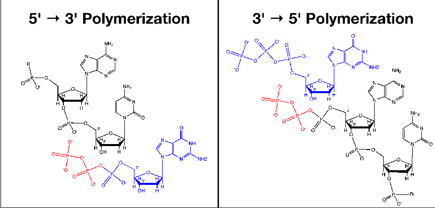
What is phenomenal about this process is that, first, it occurs in all biological organisms and, second, that it always occurs in the same manner. To understand why the consistency of directionality is notable, it helps to understand the catalytic process that occurs at the active center of nucleotide polymerases. All known nucleotide polymerases share a common chemical mechanism. In this mechanism two divalent metal cations, coordinated by a number of acidic amino acids, facilitate the transfer of an electron pair from the free 3’ hydroxyl group of one nucleotide to the α phosphate, which is attached to the 5’ hydroxyl of the other nucleotide[3] (see Figure 1.1).

Importantly, the catalytically active cations of the polymerase active site have no knowledge of whether the 5’-phosphate is attached to the incoming nucleotide or the growing chain. If one were to imagine a nucleotide polymerase that proceeded in the reverse direction of all currently known nucleotide polymerases, the only aspect of the naturally occurring enzymes that would need to be modified are those portions which attach to the growing nucleotide polymer or the incoming nucleotide, all of which are distinct from the catalytic center. That is, there should be nothing preventing the chemical reaction at a hypothetical 3′→ 5′ polymerase active site from occurring.
So the question remains: why do we not currently observe such 3′→ 5′ polymerases in nature? There are three explanations one might imagine for why no alternative polymerases are found in nature: chemical impossibility, founder effect, or evolutionary selection. Taking the first explanation, it may be that the chemistry involved in synthesis in the reverse direction, 3′→ 5′, is impossible, and only the known 5′→ 3′ polymerization reaction can be performed by biological enzymes. Yet, as noted above, catalysis does not involve segments of the growing polymer or the nucleotide monomer other than the 3’ hydroxyl and α-phosphate. If the triphosphate group were attached to the growing chain instead, and the 3’ hydroxyl group were positioned on the incoming nucleotide monomer, the active site configuration would not look any different. It is also notable that the change in entropy of the reaction would be the same regardless of polymerization reaction, as the leaving group is a pyrophosphate in either case.
The second possibility is that the unique directionality is the consequence of a founder effect. A founder effect is when a small subset of a larger population is evolutionarily isolated and goes on to give rise to a new population. This new population would be expected to contain an oversampling of the traits of the small founding population as compared to the gene frequencies of the original population[13]. In the case of nucleotide polymerization, this would imply that at some point early on in the development of life on earth the population contained both forms of nucleotide polymerase, those that polymerize by extension 3′→ 5′ and 5′→ 3′. Then, at some later point a subgroup of this population, consisting entirely of organisms with a 5′→ 3′ polymerase, was isolated and subsequently gave rise to all life on earth today.
The other possibility is that there is an evolutionary advantage to the 5′→ 3′ directionality, and that all life polymerizes nucleotides in this direction as the result of a selection event. Unfortunately, the chances of finding any evidence directly supporting the hypothesis of a founder effect determining polymerase directionality are essentially nil. Short of finding some remnant modern population with reversed polymerases, the only evidence of an ancient 3′→ 5′ polymerase would be the enzymes or other early replicator molecules themselves, and individual molecules do not fossilize. The only way to shed light on which of these two competing hypotheses explains the current state of nucleotide polymerases would be to identify an evolutionary advantage imparted by a 5′→ 3′ polymerase over the reverse.
What might be the source of such an advantage? Looking again at the chemical reactions that would be carried out in each case (fig. 1.1), a major difference between the 5′→ 3′ case and the 3′→ 5′ case is the location of the pyrophosphate leaving-group relative to the other components of the polymerization reaction. This is important because it is known that triphosphate groups attached to nucleotides can spontaneously hydrolyze[12]. In the event that the triphosphate leaves prematurely with the 5′→ 3′ polymerase, it would be possible for the enzymatic machinery to discard the (now useless) incoming nucleotide and replace it with a new nucleotide containing an active triphosphate. In the event of a spontaneous hydrolysis with the 3′→ 5′ polymerase, because the active triphosphate in the reaction is on the growing chain the only choice the enzymatic machinery has is to discard all of its progress thus far or wait for some secondary machinery to replace the triphosphate group. Given that the former of these two choices represents significant waste, we can assume that the later choice is the only one that would be even remotely sustainable, but this choice involves introducing a delay in reproduction.
A delay, on its own, does not necessarily mean that the 3′→ 5′ case is at enough of a disadvantage to be completely eliminated from a population through natural selection. After all, polymerase rates are variable and a hypothetical 3′→ 5′ polymerase could simply evolve to polymerize faster. Unfortunately, such modifications come with a cost. There is a relationship between speed of nucleotide polymerization and error rate[6], and polymerizing faster would cause the polymerase to make more mistakes. A higher frequency of errors during reproduction would introduce a higher rate of mutation, making it more difficult for the 3′→ 5′ polymerizing organisms to maintain their speed advantage. Again, on its own this is not reason enough to dismiss the possibility of a 3′→ 5′ polymerase. There are many factors at play, and to understand how all of these combined contribute to the fitness of an organism that synthesizes its nucleic acids in a 3′→ 5′ direction, we will need to model the competitive evolution of the two polymerase types.
Finally, it is easy enough to imagine a polymerase which operates in much the same fashion as modern nucleotide polymerases, but uses as its substrate nucleotides with 3′-triphosphate moieties in place of nucleotide-5′-phosphates and does not incur an excess penalty due to spontaneous hydrolysis of the triphosphate group. This hypothetical situation can be discounted, however, by considering that ribose-3-phosphate is known to decompose more readily under mildly acidic conditions than ribose-5-phosphate[9], consistent with the availability of a nucleophilic oxygen on the adjacent carbon at position 2 in ribose-3-phosphate. The implication is that the primordial pool of nucleotides would lack sufficient quantities of nucleotide-3′-triphosphates with which to do synthesis. So, we can assume that any reverse polymerase would have to work with the same nucleotide-5′-triphosphates as a 5′→ 3′ polymerase, and therefore must face the potential penalty of doing so.
Because nucleotide polymerases are responsible for replicating the genetic information of an organism and have a direct influence on both the rate at which an organism can reproduce as well as the fidelity with which genetic information is conveyed from one generation to the next, the approach we take in simulating this process is relatively straightforward. The model presented here involves simplified model organisms designed to represent the earliest forms of self-replicating life. It is assumed these organisms exist in an environment rich with nutrients and an excess of available energy. The result of this being that the rate of genome duplication serves as the lone limiting factor on reproductive rate.
Since polymerase directionality would have been fixed extremely early on in the origin of life, it is reasonable to assume that the recombination of genetic elements would contribute only a negligible amount of variation to the model organisms. Additionally, the simplest of nucleotide polymerases observed in nature are the products of single genes. Even if there was recombination of individual genetic elements, the exclusive focus of this model is the polymerase. Whether a product polymerase gene is transferred intact to the offspring of one organism or transferred horizontally will not affect the conclusions that can be made. This is a result of the first assumption made that the model organisms have an excess of all resources aside from the polymerase. That is, whatever organism a polymerase may end up in, the polymerase will always be the single determining factor for both reproductive rate and genetic fidelity.
Ultimately, the goal of this model is to investigate the link between a well understood molecular process, nucleotide polymerization, and an evolutionary outcome, the selection for polymerase enzymes which proceed 5′→ 3′. If there are general rules to be found that govern the process of evolution all the way from the molecular level to the scale of entire organisms and even populations, hopefully starting with a simple model like the one presented here will serve as an important first step in their eventual discovery.
This chapter provides a detailed description of the design of the model system used to investigate the question of the evolution of nucleotide polymerase directionality. The goal of this model is to have organisms containing either a 5′→ 3′ or a 3′→ 5′ nucleic acid polymerase compete with each other in order to see which of the strategies, if either, are evolutionarily dominant. In the model, evolutionary pressure is applied by the rate at which organisms can reproduce and the fidelity with which they duplicate their genomes. Evolutionary momentum is introduced through simple genetic mutation, which could be enabled or disabled on a per experiment basis. The model is also designed such that the influence of temperature on the outcome of this competition can be investigated.
In simplest terms, this model consists of a number of individual organisms in competition with each other. The model can be largely divided up into, and thought about most clearly as, four interacting components. These are the environment, the organisms, the genomes, and the polymerases. The relationship between these components begins with the environment. Each run of the simulation involves exactly one environment. An environment may contain many organisms, up to a predefined carrying capacity, and at the beginning of a simulation run the environment is pre-populated organisms according to a set rules.
Each organism contains one genome. At the start of an organisms “life”, it uses its genome to create a polymerase. The polymerase replicates either 5′→ 3′ or 3′→ 5′ and may not change direction. The polymerase then replicates the genome at a predetermined rate and with a random chance of introducing errors (mutations). When the polymerase is finished duplicating the genome, the organism will attempt to divide by binary fission using the newly created genome. If it is successful in doing so, then the new organism is added to the environment and begins a fresh life cycle while the original organism resets itself and also begins a fresh cycle.
A number of generalizations and assumptions have been made in order to render the problem being investigated tractable, but a consistent effort has been made to remain as true to life as possible. The motivation behind this is that, while the exact values generated by this model may not be precisely those that would be observed in the laboratory, the trends observed should hold true when transferred to the bench. For each piece decisions have been made regarding which aspects of the component are explored in depth, and which aspects are neglected, with an eye to the larger goal of investigating the role of polymerase directionality. Following is a detailed look at each component in turn.
At the start of a simulation run, the environment for that run is initialized with a starting population of organisms. To create this starting population, a set of organisms with their genome length, polymerase rate, and polymerase directionality specified is divided according each organism’s designated frequency in the starting population. The starting population size can be any number up to the specified maximum population of the environment.
A key defining feature of this model is that the environment is constrained in some ways, but not in others. Specifically, the number of organisms that can simultaneously co-exist has a hard numerical limit; a carrying capacity. On the other hand, the amount of available energy, the quantity of activated nucleotide triphosphates, and the other raw materials required for forming a cell are all considered unlimited. In reality, the carrying capacity is a generalization that could correspond to physical space limits, but it could just as easily correspond to the aggregate limitations on the other resources not explicitly modeled.
The choice of limitation based on carrying capacity was driven by two factors. The first relates to the fact that selection during an exponential growth phase could potentially operate differently than during stationary phase growth. By placing an upper limit on the size of a population, it is possible to investigate selection during both growth phases. Second, while attempting to explicitly model all of the various resource and space constraints that might ultimately limit growth might yield a more complete model, it would also significantly increase the complexity of the model without adding much insight into the question at hand. Finally, numerically or density limited growth is a common observation across a wide range of living creatures from single cells to large populations of complex animals[5].
In order to model density dependent growth inhibition as the number of organisms approaches the carrying capacity, a random death probability is introduced to the environment. In keeping with observations that the pressure of density dependent inhibition is greater as the population of an environment approaches the carrying capacity, the death probability is calculated with an inverse function of the remaining capacity

where N is the carrying capacity, n is the number of organisms currently in the environment, and 1 is added so that the probability of at least one organism being culled from the environment when the carrying capacity is reached is Pdeath = 1.
The model iterates its environment in a stepwise fashion. During each step, each of the organisms contained within the environment is allowed to carry out one time-step of its life cycle, followed by a population culling. Culling is carried out by calculating the death probability as above, and then randomly applying that probability to the environment to decide if an organism should be removed. If the decision is made to remove an organism, one is chosen from the environment randomly, removed, and the death probability is recalculated and reapplied. This process will repeat until the decision is made not to remove an organism. In this way, the number of organisms removed at each time step follows a Poisson distribution with an expectation value of Pdeath.
Organisms are created and added to the environment either at the start of a simulation run, as part of the starting population, or during the simulation run as the result of binary fission of an existing organism. If the organism is created at the start of the simulation then its genome and polymerase properties are determined by the values used to seed the population. Each of these seed organisms is generated with a random amount of its genome already synthesized, to avoid synchronization artifacts that arise if all organisms start polymerizing from zero at the start of the simulation.
If the organism is created during a simulation run, then its properties are derived from those of its parent, with the possibility of introduced variation. This variation is embodied by, and in the model determined by, the genome contained within the organism. Each organism contains exactly one genome and one polymerase. Having only one polymerase is a simplification, but it is justified by considering this one polymerase as an exemplar of all the polymerase enzymes that would be found in a real organism.
Each organism is modeled as a state machine. The two states in which an organism can exist are: Polymerizing or Duplicating. At creation, each organism starts in the Polymerizing state. When an organism is in the Polymerizing state, each simulation time-step is used to allow the organism’s polymerase to add nucleotides to the genome copy being constructed. At the end of each time-step, the polymerase is queried as to whether or not it is finished with constructing the nascent genome. If it is, then the organism shifts to the Duplicating state. Otherwise, it remains in the Polymerizing state.
When an organism reaches the Duplicating state, a check is performed to determine if the genome copy constructed by the polymerase is viable. This is a simple sanity check to ensure that the synthesized genome is of the correct length. If the genome copy is not viable, then it is discarded and the organism returns to the Polymerizing state to create a new genome copy. If the genome is viable, the next determination that must be made is whether or not there is available capacity in the environment for a new organism.
If the number of organisms in the environment is not at the environment’s carrying capacity at the start of a simulation time step, then an organism in the Duplicating state can proceed to create a new organism. The thus created organism containing the newly synthesized genome is inserted into the environment. In this case, the parent organism will return to the Polymerizing state to begin construction of yet another new genome. If, instead, the environment is at capacity at the start of a simulation time step, then any organism in the Duplicating state will remain unchanged, in the Duplicating state. It will next attempt to add a new organism with the synthesized genome during the next environment step.
Genomes are created before the organism in which they are contained. In the case of a running simulation, the new genome is created by the parent organism before binary fission. For the starting population of organisms used to seed a simulation, the genomes are created ahead of time with predefined properties and a random amount of replication already completed. The model genomes perform three important functions for the simulation: they generate polymerases with properties defined by the genome, they track the progress of the organism’s polymerase during polymerization, and they return a copy of themselves once polymerization has completed.
Each genome codes for either a 5′→ 3′ polymerase or a 3′→ 5′ polymerase, and this will not change through subsequent generations. There is the possibility that this is not perfectly reflective of how early organisms may have functioned, as it is conceivable that, through acquired mutations, a genome which coded for a 3′→ 5′ polymerase may evolve in subsequent generations into a genome that codes for a 5′→ 3′. Were this to occur, it would either have to be through a gradual mechanism or a small mutation affecting global properties of the polymerase. A gradual mechanism would be one where the forward or reverse speed of the polymerase is reduced to nearly zero, and then eventually the directionality flipped. It is safe to eliminate this possibility in the model, as such a transition would require the survival of an organism with an especially slow polymerase. As a consequence of the starting assumption that polymerase speed is the primary determining factor in the speed of replication, such organisms would be quickly out-competed in the simulation.
The alternative mechanism of a small mutation leading to a global change can also be neglected for two reasons. First, if such a mutation were possible, the fidelity of communicating polymerase directionality from one generation to the next would be diminished. This would imply that selecting against a 3′→ 5′ polymerase would effectively be impossible, as such polymerases could appear at almost any time. This would also narrow the window of possible founder populations were the alternate founder effect hypothesis considered. In the case that polymerase directionality were trivially reversible, the hypothetical founder population would not only have to be homogenous in their polymerase directionality, but they would also have to have a unique restriction on the directionality reversing randomly. This also highlights the second reason that the possibility of such a mutation need not be considered: if such mutations were possible, it would be expected that they could be observed today. Certainly, it is possible that such a mutation might have existed in the past but have subsequently been locked out of the population of current polymerase sequences, but this seems unlikely. Nucleotide polymerases are wildly variable in their sequence and structure throughout all forms of life, and yet none exhibit reversed directionality.
When a genome is asked by its organism to create a polymerase, it will imbue the polymerase with a fixed polymerase rate in addition to a fixed directionality. The precise value the polymerase speed will take is determined when the genome is created from its parent (or from predefined values at the beginning of a simulation). Once the polymerase has been generated and polymerization begun, the polymerase will inform the genome during each simulation time-step how many nucleotides have been added to the copy being created, and how many of those are erroneous base pairs. The genome keeps track of this information for later reporting and calculations.
When a genome copy is constructed, the genome can then provide that copy to a new organism, but in doing so it must determine the properties of this new genome. As mentioned above, the directionality is inherited exactly. The polymerase speed coded for by the copy genome is determined in a two step calculation based on the number of errors (mutations) introduced. First, the variance from the parent genome’s encoded polymerase rate is calculated by taking

where rmax and rmin are the maximum and minimum possible rates, respectively, M is the
number of errors made during replication, taken as a fraction of total genome length, and
Mmax is the maximum tolerated fraction of errors, which was set at  . The maximum
tolerated fraction of errors is the threshold above which it can be assumed that the
inherited traits of the polymerase are, essentially, selected at random. The maximum
and minimum rates were chosen as 1 and 10 nucleotides added per simulation
time-step to reflect the roughly 10-fold range of empirically observed polymerase
rates.
The logic behind this metric is that more mutations will, on average, lead to greater alteration of enzyme function. Certainly there are individual mutations that could, on their own, have a large effect on polymerase rate, but averaged over many polymerases and many possible mutations, this general trend should hold. Once the variance is determined, it must be applied to the parent genome’s encoded polymerase rate in such a way that the child’s genome does not code for an invalid polymerase. So, if the variance would generate a polymerase rate above the maximum, then it is subtracted from the parent rate, and vice versa. If the variance would not result in an invalid rate as a consequence of either addition or subtraction, then it is applied to the parent rate with an equal probability of either outcome.
The single most significant component of the model is the model nucleotide polymerase itself. The other three components described above serve primarily to ensure that selection and descent with modification will occur, but it is the polymerase which embodies the trait that is ultimately being selected for or against: the polymerase’s directionality. As with the genomes, the directionality and rate of a polymerase does not change subsequent to its creation. These properties are determined by the genome from which the polymerase is generated. The polymerases only have one function during a simulation: to add nucleotides to a growing genome copy. How this occurs depends on the polymerase directionality and the temperature of the simulation.
When an organism in the Polymerizing state carries out one step of simulation time, the polymerase will add nucleotides to the genome being synthesized. The polymerase does this by running through a loop with a maximum number of iterations determined by its rate. So, for example, a polymerase with a rate of 7 can carry out its nucleotide addition loop a maximum of 7 times for each 1 simulation time step. During each loop, two determinations must be made. First, the polymerase must determine whether the nucleotide about to be added is activated, and second it must determine whether a properly base-paired nucleotide is being added, or whether the nucleotide being added will generate a replication error.
The reason that the polymerase must determine whether or not the nucleotide being added is activated is due to a consequence of chemistry. All known nucleotide polymerases in nature use, as their substrate, nucleotide triphosphates. They use the energy released by cleaving the bond between the α and β phosphates attached to their 5′ carbon to drive the polymerase reaction forward. However, this bond can be cleaved through spontaneous hydrolysis by water. The equilibrium between active and inactive nucleotides can be described by a Boltzmann distribution:

where ΔG0 is the standard free energy of the hydrolysis reaction. To simplify the
simulation calculations, the entire  term is expressed as a generic simulation
temperature
  .
.
Where this process of inactivation becomes important is in how it will differentially affect a 5′→ 3′ polymerase vs a 3′→ 5′ polymerase. In the 5′→ 3′ case, the one that is observed in all known forms of life, the triphosphate is attached to the incoming nucleotide about to be added to the chain. If this incoming nucleotide becomes inactive before the polymerase has a chance to join it to the growing nucleic acid polymer, then this represents a wasted addition step. That is, if a polymerase with a rate of 7 has one of its nucleotides become inactive before phosphodiester bond formation, then it will only add 6 nucleotides during this simulation time-step.
On the other hand, in the case of a hypothetical 3′→ 5′ polymerase, the triphosphate group would be attached to the 5′ carbon of the nascent nucleic acid polymer. If this triphosphate is cleaved during an addition step, the polymerase will not be able to compensate by drawing in a new nucleotide from the pool of available nucleotides. Rather, the polymerization process will necessarily halt while the terminal end of the growing chain is reactivated. In the simulation, that process is modeled by terminating the polymerase’s addition of new nucleotides when an inactivation event occurs. That is, if a 3′→ 5′ polymerase with a rate of 7 experiences inactivation during the addition of the 3rd nucleotide in this time step, then only 2 new nucleotides will be added to the growing genome during this particular step.
Furthermore, whereas a 5′→ 3′ polymerase will be constantly drawing in new, activated nucleotides from the pool of all available nucleotides, a 3′→ 5′ polymerase depends on the nascent chain remaining activated. The consequence of this is that the probability of a 5′→ 3′ polymerase experiencing a deactivation event depends only on the free energy of the reaction and temperature, irrespective of polymerase rate. Alternatively, a 3′→ 5′ polymerase runs a greater risk of the triphosphate on the nascent chain becoming deactivated the longer it waits before adding a new nucleotide. So, for the reverse polymerases, the distribution was adjusted by a factor determined by the polymerase rate:

where rmax is the maximum polymerase rate and r is the rate of the polymerase doing the addition. This extra factor accounts for the fact that a slower reverse polymerase will give each terminal phosphate group on the growing chain a longer period of time before addition of the next nucleotide monomer during which a spontaneous hydrolysis might occur.
Finally, each time a new nucleotide is added by a polymerase, there is a risk that the nucleotide will be of the wrong sort. The primary driving force discriminating properly base-paired nucleotides from improperly paired nucleotides is the formation of hydrogen bonds between the incoming nucleotide and the corresponding nitrogenous base of the template nucleic acid. The hydrogen bond interaction that allows discrimination between Watson-Crick base-pairing and a variety of mismatches was modeled using the same sort of Boltzmann distribution as used for the spontaneous hydrolysis condition. However, since the ΔΔG0 of a correct versus incorrect base pairing is twice that of the spontaneous hydrolysis reaction[11, 1], the hydrogen bond portion of the erroneous inclusion calculation is made using the formula:

where t is the simulation temperature.
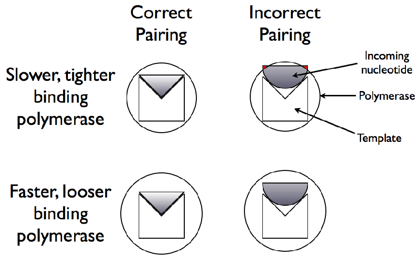
Recently, research has indicated that hydrogen bond formation is not sufficient to completely explain the fidelity of correct pair formation by nucleotide polymerases. It has been suggested that polymerases also take advantage of geometric differences between proper and improper pair formation to improve their ability to discriminate correct versus incorrect base pairing. Prior studies have revealed a relatively complex link between polymerase rate and error rate for nucleotide polymerases[2]. The essence of this link is that there is an additional geometric constraint on erroneous nucleotide inclusions and that, in order to polymerize faster, polymerases must relax this constraint.
In the model, this additional factor is treated as a simple flow problem. If a polymerase is roughly represented as a cylindrical tube, the narrower the tube is the greater will be its ability to reject geometrically unfavorable nucleotide pair configurations. However, the rate of the polymerase will also be affected by the radius of the tube (see figure 2.1 for an illustration of this concept). If rate is taken as the flux of nucleic acid through the tube, then we end up with a simple square root relationship between the ability of the polymerase to reject based on geometry and the number of nucleotides it can add in one simulation time-step. Specifically

describes the geometric discrimination and

is the probability of making a mistake during each nucleotide addition event, calculated as the product of the temperature dependent Boltzmann distribution, K, and the geometric discrimination function, Γ. Alternatively, in order to investigate the effect of mutation on evolution, Perror could be artificially set to 0 at the start of a simulation run.
The procedure for performing an experiment with the model for polymerase directionality evolution consists of constructing an environment for the model to operate on, then setting the model running for a set number of time steps. Various parameters of the simulation are reported at set intervals during the run. Because a number of the dynamical systems in the model depend on randomly generated numbers, each experiment was carried out in 10 copies to smooth fluctuations, and all of the values reported represent a numerical average of all 10 runs. All plots were generated using the R software package[7].
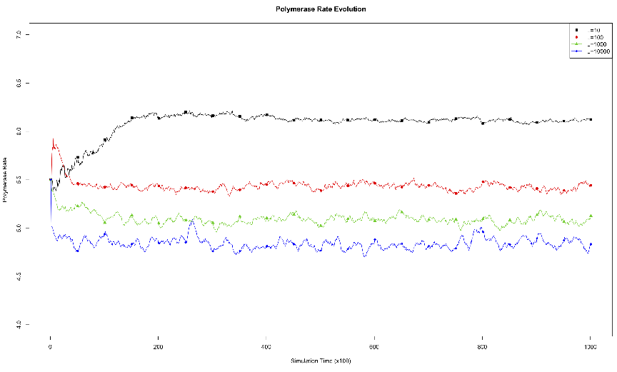
The dynamics included in the model for polymerase directionality should generate scale free results. That is, the evolution of traits should show the same dynamics regardless of population size or genome length. In this model, the only trait capable of evolving is polymerase rate, so in order to verify that the dynamics were indeed scale free, the first experiments carried out were designed to investigate simple dynamics of polymerase rate evolution over a range of scales. One experiment consisted of starting populations of 10 organisms and a maximum population (environmental carrying capacity) of 1000 organisms combined with 4 different genome lengths as described in table 3.1.
| Temp. (t) | Starting Pop. | Max Pop. | Genome Length |
| 0.40 | 10 | 1000 | 10 |
| 0.40 | 10 | 1000 | 100 |
| 0.40 | 10 | 1000 | 1000 |
| 0.40 | 10 | 1000 | 10000 |
In order to avoid a founder bias with regards to polymerase rate, in each experiment the ten organisms in each seed population consisted of one organism of each of the ten possible polymerase rates. The simulation temperature of 0.40 was chosen because it results in a significant amount of error, and therefore variability due to mutations, during growth but is not a high enough temperature that certain other temperature effects begin to alter growth and evolution. The results from this experiment are plotted in figure 3.1.
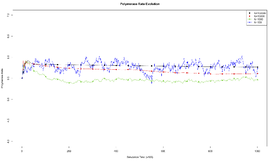
Second, a set of experiments were carried out to investigate the effect of population size on the evolution of polymerase rate. In this experiment, the genome length of the organisms in each environment was held constant at 1000, the starting population was set to 10, and the maximum population was set to either 100, 1000, 10000, or 100000. As in the first set of experiments, the starting population in each environment was seeded with organisms with polymerase rates evenly distributed in the range 1-10 and the simulation temperature was set to 0.40. Table 3.2 summarizes these experiments.
| Temp. (t) | Starting Pop. | Max Pop. | Genome Length |
| 0.40 | 10 | 100 | 1000 |
| 0.40 | 10 | 1000 | 1000 |
| 0.40 | 10 | 10000 | 1000 |
| 0.40 | 10 | 100000 | 1000 |
Figure 3.2 is a plot of the average polymerase rate of the population in each environment against the simulation time. Based on these initial experiments, it was decided that a maximum population size of 1000 with a genome length of 1000 could serve as an adequate representative of the dynamics over the range of possible values. These values were chosen because they also keep the size of the simulations reasonable with regards to the amount of computational time required to run each simulation, since the run time of the simulations scale with the population size and organisms with longer genomes require more time-steps to achieve the same number of doublings as organisms with shorter genomes.
Finally, in order to validate the model and how reasonably it simulates the observed growth dynamics of biological organisms, a set of experiments were carried out starting with small populations of 10 organisms, as before, and following their growth at different temperatures. The first two sets of experiments described above were only carried out with forward polymerizing organisms. To be sure that model organisms with reverse, 3′→ 5′, polymerases had growth dynamics similar to forward polymerizing organisms, these experiments were carried out using both types of organisms. Table 3.3 summarizes the parameters used for these experiments.
| Temp. (t) | Max Pop. | Genome Length | Directionality |
| 0.10 | |||
| 0.30 | forward | ||
| 0.40 | 1000 | 1000 | |
| 0.60 | |||
| 0.10 | |||
| 0.30 | reverse | ||
| 0.40 | 1000 | 1000 | |
| 0.60 | |||
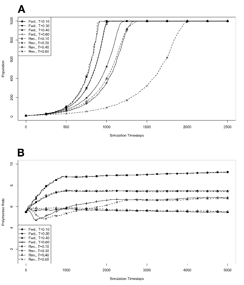
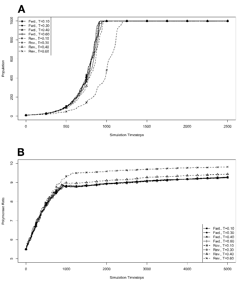
The results of these simulations are presented in figure 3.3. Simulations were carried out for each type of polymerase individually so that only the dynamics of the polymerase would influence growth. The simulations were also run disallowing mutations. Under this condition there can be no change in polymerase rate for an individual and its daughters from one generation to the next. These results are presented in figure 3.4. We monitored both the population rate and the average polymerase rate for all the organisms in the environment.
 .
.
 .
.
In each of the experiments performed up to this point, forward or reverse organisms were allowed to grow in isolation. In order to gain some insight into the dynamics of polymerase evolution, it is necessary to set these two classes of model organisms in competition with each other. When considering the competition of organisms, there are two domains which are interesting to probe. The first is the competition of the organisms as they explore a new ecological niche. That is, the way in which organisms compete during phases of exponential growth. The second is the competition that occurs when an environment is already at its carrying capacity. It would be expected that an evolutionary strategy which results in the most rapid growth should dominate during exponential growth. It is also conceivable that such a strategy might not represent the most efficient use of resources available and therefore might ultimately loose out to a different strategy when growth is limited by resources.
We investigated how organisms with forward or reverse polymerases would behave when competing with each other for resources during an exponential growth phase. To do this, we seeded environments with 100 organisms, where 50 of the organisms contained forward polymerases and 50 reverse. For each type, there were 5 organisms with each possible polymerase rates for an average starting polymerase rate of 5.5. Table 3.4 summarizes the parameters used for these experiments.
| Temp. (t) | Max Pop. | Genome Length | Seed organisms |
| 0.10 | 50 forward | ||
| 0.30 | and | ||
| 0.40 | 1000 | 1000 | 50 reverse |
| 0.60 | |||
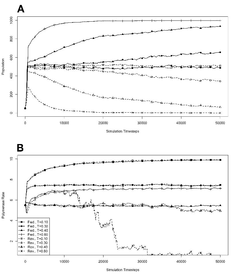
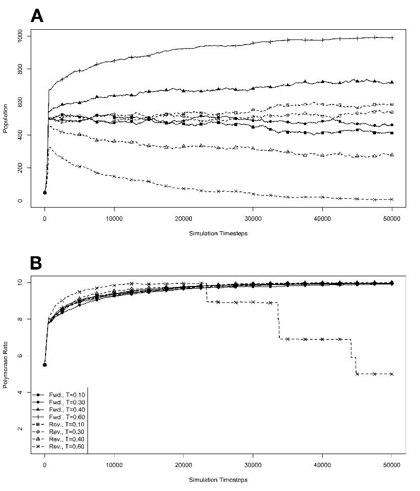
The results of these simulations are presented in figure 3.5. Simulations were again replicated disallowing mutations. These results are presented in figure 3.6. In each environment, we tracked the subpopulations of organisms with forward and reverse polymerases separately so that we could follow the population changes and polymerase rate evolution for each condition in the mixed case independently.
 .
.
 .
.
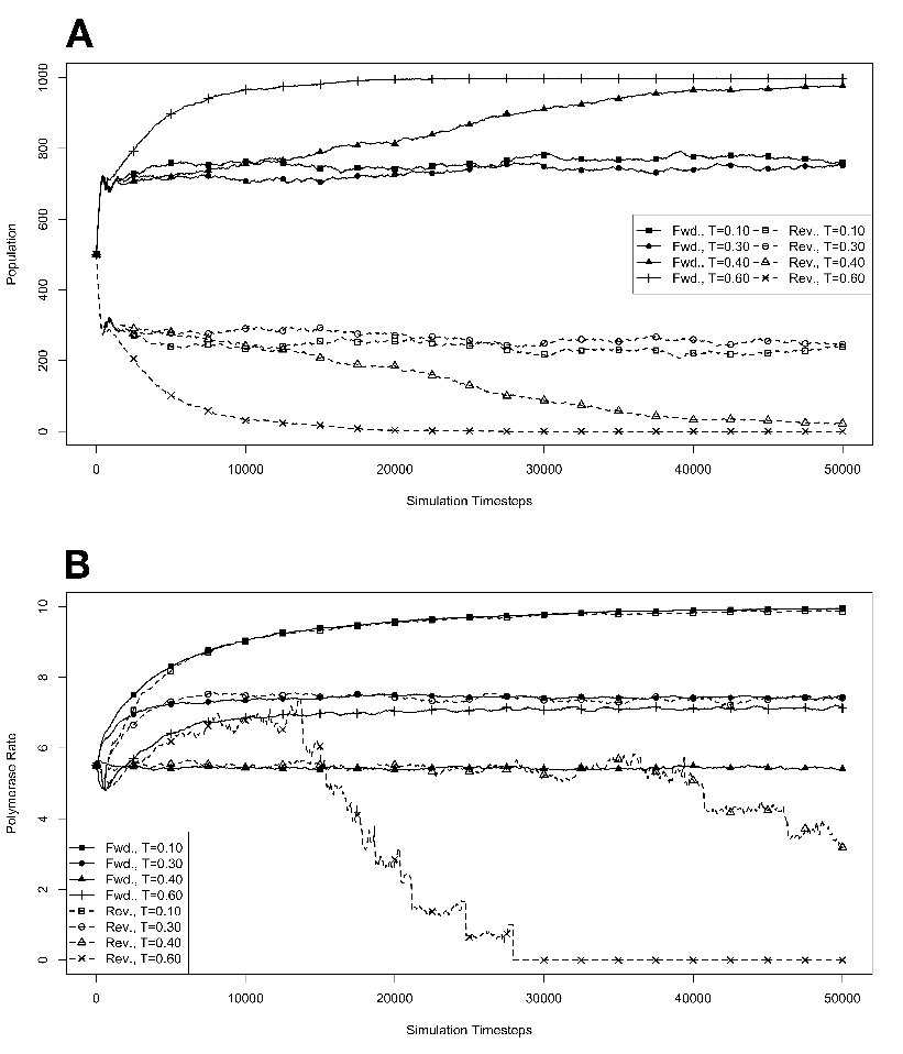
To further investigate how organisms with forward polymerases fared in competition with organisms with reverse polymerases, specifically to see if an equilibrium was possible between the two varieties, we performed a number of simulations starting with an environment already at its maximum capacity. This was done by seeding each environment with 500 organisms containing forward polymerases and 500 containing reverse. For each variety, there were 50 organisms seeded with each of the 10 possible polymerase rates. Table 3.5 summarizes the parameters used for these experiments.
| Temp. (t) | Max Pop. | Genome Length | Seed organisms |
| 0.10 | 500 forward | ||
| 0.30 | and | ||
| 0.40 | 1000 | 1000 | 500 reverse |
| 0.60 | |||
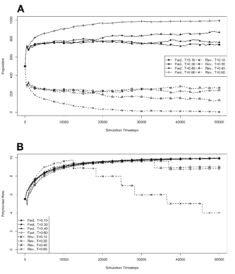
The results of these simulations are presented in figure 3.7. As before, these conditions were repeated with mutations disallowed, and those results are presented in figure 3.8.
 .
.
 .
.
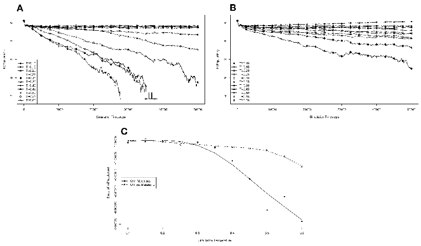
We noted that the results of this last experiment seemed to indicate that, when mutations were allowed, their might be a temperature regime in which there is a transition between an equilibrium of organisms containing forward and reverse polymerases and a complete dominance by organisms containing the forward polymerase. To get a more detailed picture of this transition temperature, we repeated the simulations with full environments at temperatures from 0.10 to 0.60 in 0.05 increments. Table 3.6 summarizes the parameters used for these experiments, and figure 3.9 shows the results of these simulations.
| Temp. (t) | Max Pop. | Genome Length | Seed organisms |
| 0.10 | |||
| 0.15 | |||
| 0.20 | 500 forward | ||
| 0.25 | |||
| 0.30 | |||
| 0.35 | 1000 | 1000 | and |
| 0.40 | |||
| 0.45 | |||
| 0.50 | 500 reverse | ||
| 0.55 | |||
| 0.60 | |||
In the study of evolutionary dynamics there exists the concept of a stable equilibrium. The organisms in such a situation may not all represent the “best fit” mechanism for coping with a particular ecological niche, but at the same time none are sufficiently better off than the others that they will dominate the population. If organisms polymerizing nucleotides in a 3′→ 5′ direction represented a stable equilibrium with organisms polymerizing in a 5′→ 3′ direction, then it would be expected that organisms exhibiting such a trait should be found in nature. On the other hand, if 3′→ 5′ polymerization is a loosing strategy when in competition with 5′→ 3′ polymerization, the lack of modern 3′→ 5′ polymerizing organisms would be an expected consequence of Darwinian evolution.
When modeling the competition between organisms with a 5′→ 3′ polymerase and organisms with a 3′→ 5′ polymerase, this is an important aspect of modern evolutionary theory to keep in mind. It is not sufficient to show that polymerizing nucleotides in a 5′→ 3′ direction is better fit than, or produces organisms which reproduce faster than polymerizing nucleotides in a 3′→ 5′ direction. Rather, to discriminate between the possibility that the modern ubiquity of 5′→ 3′ polymerases is the result of a founder effect versus being a consequence of natural selection, we need to show that 3′→ 5′ polymerizing organisms cannot exist in a stable equilibrium. It is with this in mind that the model presented here was constructed.
In constructing this model, a number of explicit and implicit assumptions were made. The first, and perhaps largest, assumption is that polymerizing nucleotides to create new nucleic acid polymers by adding nucleotide triphosphates to the 5′ end of the growing chain is physically possible. As there are no known polymerase enzymes which carry out the polymerization reaction in a 3′→ 5′ direction, it is impossible to say with certainty that such polymerases might exist. However, based on the nature of the active site chemistry of nucleotide polymerases, there is also no reason to believe that such 3′→ 5′ polymerases are not possible, beyond the fact that such polymerases do not currently exist. For this reason, we are comfortable with this assumption.
The second implicit assumption made in constructing this model is that the only viable building blocks for nucleic acid polymers are 5′-triphosphate nucleotides. If nucleotides phosphorylated on their 3′ oxygen could be used by a hypothetical 3′→ 5′ polymerase, then the chemistry of such a polymerase would not, qualitatively, be any different than that of a 5′→ 3′ polymerase working with 5′-triphosphate nucleotides. That is, in the case that a 3′→ 5′ polymerase could work with a 3′-triphosphate nucleotide, then the activated triphosphate moiety would reside on the incoming nucleotide, instead of on the growing chain, in the same way that the triphosphate moiety is found on the incoming 5′-triphosphate nucleotide used by 5′→ 3′ polymerases.
We can discount the possibility of 3′-triphosphate nucleotides as raw material for a polymerase reaction for a number of reasons. If, in keeping with current scientific consensus, ribonucleic acids represent the more ancient form of nucleotides and the 2′-deoxyribonucleic acids are a more recent invention of biology, then a potential 3′-triphosphate nucleotide would have its triphosphate group attached on a carbon adjacent to a free hydroxyl. The free 2′-hydroxyl group of ribonucleic acids is known to polymerize hydrolysis reactions in a number of ribozymes, so it would not be unreasonable to assume that the 2′-hydroxyl would also catalyze a hydrolysis of the triphosphate group on a 3′-triphosphate nucleotide. This would serve to significantly restrict the available primordial pool of 3′-triphosphate nucleotides as compared to 5′-triphosphate nucleotides, whose adjacent carbon’s oxygen would normally be incorporated in the formation of the furanose ring. Indeed, it has been shown that ribose-3′-phosphate decomposes more readily under mild acid conditions than ribose-5′-phosphate.
The remaining assumptions made are the various explicit assumptions required for construction of the model itself as described in chapter 2. Of these, the most important is the assumption that the dynamics of spontaneous nucleotide hydrolysis occur on a time-scale commiserate with the time-scale of nucleotide incorporation and the assumption of a geometry-based discrimination mechanism for incorrect nucleotide incorporation by the polymerase. We can surmise that the time-scale for spontaneous nucleotide hydrolysis cannot be significantly smaller than the time-scale for nucleotide incorporation, for if it were then nucleotide polymerization would, in effect, be impossible. If the time-scale were much larger, this would be the equivalent of removing a constant factor from the calculation for the probability that nucleotide inactivation occurs during polymerization. The effect of such an adjustment would be largely quantitative, raising the simulation temperature at which the effects reported would be observed.
A note should be made on the significance of the simulation temperature used in the
model. If we take the expression used in the model for the temperature dependence of the
equilibrium between the polymerase-template-nucleotide complex for the correct
nucleotide, the free polymerase-template complex, and the polymerase-template-nucleotide
complex for the incorrect nucleotide: e- , and compare it to the experimentally determined
value of 5
 for the ΔΔG of this system, we can calculate the real temperature
corresponding to each simulation temperature with the expression

This gives us a real temperature of -22∘C for a simulation temperature of 0.10 and a real temperature of 1200∘C for a simulation temperature of 0.60. Obviously this range of temperatures is unreasonably large for life, even when accounting for aqueous environments with high salinity or at high pressures.
As mentioned in the introduction, every effort was made when designing this model to remain faithful to the realities of the biochemical processes that a nucleotide polymerase must carry out. That said, a number of confounding factors limit the applicability of the precise quantitative temperature values used in the simulations to understanding real biological processes. It has already been mentioned that the need to reduce the probability of spontaneous nucleotide hydrolysis by a constant factor to account for a difference in time-scales would effect the absolute temperature values at which various simulation outcomes are observed. The same sort of constant factor consideration would, potentially, also need to be made to account for a difference between the precise effect of geometry-based discrimination of real nucleotide polymerases and the model values.
The primary model values impacted by simulation temperature are those for the equilibrium describing the incorporation of correct versus incorrect nucleotides during nucleic acid synthesis, and the equilibrium between active and inactive nucleotides. The chemical phenomena described by these values, however, are subject to more influences than just temperature. For example, it is well documented that the energy associated with a correct nucleotide base-pairing is heavily influenced by the dielectric constant of the solvent and the concentration of nucleic acid counter-ions. The equilibrium of nucleotide triphosphates would, likewise, be subject to influence by effects of nucleotide concentration and pH. Thus, the value of simulation temperature can be thought of as a stand in for a number of thermodynamic factors that might influence the biochemical processes involved in the model processes. Therefore, the primary utility of the simulation temperature is in revealing the collected influence of thermodynamics on the system. Before we consider these influences, let us look at the results of the initial experiments performed with the model.
In constructing the model presented here, we were attempting to evaluate the plausibility of the hypothesis that all life contains nucleotide polymerases which proceed in a 5′→ 3′ direction due to an evolutionary advantage of this mechanism versus the reverse 3′→ 5′ direction. In order to address this question while still remaining biologically relevant, it was necessary to account for a pair of temperature dependent chemical processes: spontaneous hydrolysis of nucleotide triphosphates and inclusion error rate.
First, to validate the kinetics of the model we carried out a number of simulations in which each sort of organism, those containing the 5′→ 3′ (forward) polymerase and those containing the 3′→ 5′ (reverse) polymerase, were allowed to grow from a small starting population in the absence of competition (fig. 3.3A). These experiments revealed that the temperature of the environment had a gradual impact on the growth rate of the model organisms, with the greatest inhibition on growth rate occurring at the highest temperatures investigated. At these higher temperatures, the effect on growth appeared to be greater on organisms containing the reverse polymerase than on those containing the forward polymerase. This indicates that the disadvantages inherent in polymerizing nucleic acids in a 3′→ 5′ direction become more exaggerated as the temperature increases.
Another way to analyze these experiments is to look at the way that the rate of the nucleotide polymerases evolves at each temperature. Generally, we can state that tendency toward a faster polymerase indicates that the predominant evolutionary pressure is on reproduction rate, while a tendency toward slower polymerases indicates an increased importance of reducing the mutation rate. This stems from the fact that a faster polymerase will have a greater error rate. With this in mind, figure 3.3B shows that, as the temperature of the simulation increases, the average polymerase rate decreases indicating the increasing importance of avoiding errors. This is true up to simulation temperatures of 0.40, but at a simulation temperature of 0.60 the trend reverses indicating a switch back toward reproduction rate as the primary evolutionary pressure.
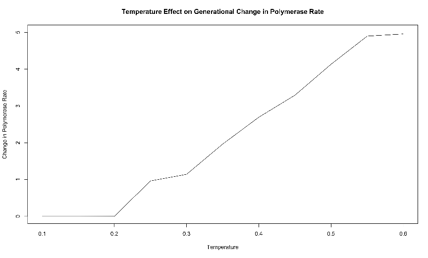
This switch most likely represents a saturation of the effect that mutation can have on the organisms. That is, in our model system an increasing mutation rate decreases the fidelity with which each generation can pass along its traits (in this case just polymerase rate) to subsequent generations. We expect that, at some high mutation rate, this fidelity drops significantly enough that the polymerase rate inherited from one generation to the next is not significantly distinguishable from a randomly assigned value. When the temperature of the simulation gets high enough, the error rate due to the thermal component will overwhelm the error rate due to polymerase rate, and reach this critical value. At this point the selective pressure against faster polymerases resulting from the need to preserve generation to generation fidelity will, in effect, vanish. In our system, this leaves growth rate as the single remaining selective pressure, explaining the reversal of the trend of polymerase rate evolution at high simulation temperatures. Indeed, as can be seen in figure 4.1, at simulation temperatures of 0.55 and 0.60, the average change in polymerase rate from one generation to the next is nearly 5, the maximum that would be expected if polymerase rates were inherited at random.
One interesting result from this first experiment that was not completely anticipated was that the polymerase rate of the forward and reverse polymerizing organisms would be so similar over a wide range of simulation temperatures. We expected that reverse polymerizing organisms, with the increased penalty for a spontaneous hydrolysis event, would have a greater selective pressure to evolve a faster polymerase holding all else constant. This seems to not be the case, though, as the average polymerase rate of the forward and reverse polymerizing organisms at all but the highest temperature are indistinguishable. The only conclusion we can draw from this observation is that the selective pressure on mutation rate is sufficiently rigid enough to make the spontaneous hydrolysis penalty a negligible influence on the evolution of polymerase rate. This conclusion is further backed up by evidence from the simulations with no mutation allowed, as described below.
The next set of experiments was intended to look at how forward and reverse polymerizing organisms would fare in competition with each other at various temperatures. We again started each simulation with a small seed population and allowed these populations to grow in an exponential fashion. As we expected based on the similarity of growth rates for the forward and reverse polymerizing organisms growing in isolation, both forms grew rapidly until the environment was at capacity with approximately half of the population belonging to each form. At this point, competition kicks in and at simulation temperatures of 0.1 an equilibrium between the two forms is established. At a simulation temperature of 0.3, it is unclear in the duration of the simulation run whether an equilibrium might eventually be established or whether the reverse polymerizing organisms would eventually be outcompeted. At the higher simulation temperatures of 0.4 and 0.6, the reverse polymerizing organisms are outcompeted by the forward polymerizing forms, however at the temperature of 0.4 this is a true out-competition, where the reverse polymerizing form grew to occupy nearly half the population before being eradicated. At a simulation temperature of 0.6, the reverse polymerizing organisms are never able to establish themselves.
At the higher temperatures, the average polymerase rate of the reverse polymerizing organisms begins to drop off as their population numbers, as seen in figure 3.5B, begin to drop off. This drop is not, however, indicative of a reduction in the fitness of the reverse polymerizing organisms. Rather, as the reverse polymerizing organisms are gradually outcompeted by the forward polymerizing organisms their number is reduced. Since the only mechanism in the model for removing organisms from the population is the density dependent random culling, which members of the reverse polymerizing organism population will be removed is likewise random. Since the organisms with a faster polymerase rate will reproduce more rapidly, they will be present in greater number, and therefore will be more likely to be removed from the environment first. In other words, the rate of the decrease in average polymerase rate of the reverse polymerizing organisms can be seen as a proxy measure for the rate at which the forward polymerizing organisms are preferentially occupying the available capacity in the environment created when a reverse polymerizing organism is culled.
Looking at the evolution of the polymerase rates of the forward and reverse polymerizing organisms, it is apparent that the selective pressure on polymerase rate is greater when there is competition involved at low temperatures. That is, at a simulation temperatures of 0.3 and 0.4, the steady-state polymerase rate under competition is not appreciably different than under the no competition growth case, but at a simulation temperature of 0.1 the steady-state polymerase rate under competition is elevated as compared to the average polymerase rate for both forward and reverse polymerizing organisms growing in isolation. From this we can conclude that rapid growth takes on an increased importance when competition with an alternative strategy is involved.
Because the reverse polymerizing organisms were not able to grow significantly at a temperature of 0.6 under competition, and because of the ambiguity of the eventual fate of the reverse polymerizing organisms at a temperature of 0.3, we were curious what might happen if both forms started off at a significantly larger population size. Specifically, we were interested to see if forward polymerizing organisms represented an evolutionarily stable strategy at these temperatures[10, chap. 4]. In order to investigate this question, we carried out simulations starting with completely full environments split evenly between forward and reverse polymerizing organisms at various temperatures.
The results from these simulations (fig. 3.7) indicate that the ultimate success of the forward and reverse strategies in competition with each other when starting from half of an environment at capacity is similar to that during exponential growth, though the dynamics are interestingly different. In general, we can conclude that forward and reverse polymerizing organisms will establish an equilibrium at lower temperatures and that forward polymerizing organisms are dominant at higher temperatures. That is, at sufficiently high enough temperatures, polymerizing nucleotides in a 5′→ 3′ direction appears to be an evolutionarily stable strategy.
Also, the steady state polymerase rates reached at each temperature are the same as
for the exponential growth case above. The simulations starting with a full population
differ from those starting with exponentially growing populations in how the steady state
is reached. Arrival at the steady state polymerase rate occurs much earlier in
the case of exponential growth. This reflects the fact that in a mostly empty
environment it is easier for the best fit organisms to rapidly dominate a population. In a
population already at capacity, this rebalancing of traits can only occur through
attrition, which is a more gradual process. Interestingly, the rate at which the
steady state polymerase rate is achieved appears to impact the distribution of the
equilibrium population. At a simulation temperature of 0.1, the equilibrium population
in the exponential growth case is evenly divided between forward and reverse
polymerizing organisms, but in the full environment case the split is closer to  forward
polymerizing organisms and
  reverse. We believe that this difference may point toward
the existence of different domains of competition. That is, it may be possible
that the fitness of the model organisms is impacted by the population relative
to the environment’s carrying capacity. Since there are two fitness components
encoded in the polymerases of our model organisms, namely proliferation rate
and mutation rate, what we may be observing is the existence of multiple fitness
equilibria between the forward and reverse polymerizing organisms. Future models
wherein these fitness components could be decoupled might help resolve this
possibility.
To better understand the role that mutation and the introduction of random variation from generation to generation might have on the results of our simulations, we modified the model system to remove the possibility for mutation. With this modification, the average polymerase rate can still evolve, but only through selection of individuals. Also, since the only evolutionary pressure acting on the model organisms is reproduction rate, we would expect that all individuals should converge on the maximum polymerase rate. Indeed, this is precisely the result we observe (fig. 3.4B). With the selective pressure of mutation removed, we can also directly observe the impact of the penalty on reverse polymerizing organisms due to spontaneous hydrolysis of nucleotide triphosphates. In figure 3.4B, we can see that at simulation temperatures of 0.4 and 0.6 the reverse polymerizing organisms evolve to faster polymerase rates sooner than their forward polymerizing counterparts.
We also note that the exponential growth of both the forward and reverse polymerizing organisms is essentially identical at all temperatures except for 0.6 (fig. 3.4A). Reverse polymerizing organisms at a simulation temperature of 0.6 are the only group to deviate. This is due to the excessive penalty paid by a reverse polymerase at this high temperature. Moreover, the reverse polymerizing organisms at a simulation temperature of 0.4 appear to grow with identical kinetics to the forward polymerizing organisms at this temperature, showing that the penalty of a reverse polymerizing strategy can be compensated for by evolving a faster polymerase (as seen in fig. 3.4B).
Following this initial result, we then repeated the prior experiments starting with small populations and starting with a full environment, but with mutations disallowed (figures 3.6 & 3.8, respectively). When we start with small populations we see, as before, that polymerase rate rapidly evolves to its equilibrium value (fig. 3.6B). The difference here is that without mutation this equilibrium value at all temperatures is the maximum polymerase rate allowed. At the highest temperature of 0.6, the reverse polymerizing organisms are unable to establish themselves the same as when mutations were allowed, implying that this inability to compete with forward polymerizing organisms during exponential growth is a consequence of the spontaneous hydrolysis penalty and is not affected by the presence or absence of mutations in the system.
Paying attention to the way that the competition between forward and reverse polymerizing organisms resolves itself at a simulation temperature of 0.4 when starting with a small population (fig. 3.6A), its not entirely clear whether an equilibrium between these forms can be established. If we look for the establishment of an equilibrium when starting with a full environment at the same temperature (fig 3.8A), it does appear that the forward polymerizing organisms are outcompeting the reverse polymerizing organisms, but the rate at which this take over happens is definitely slower than when mutations are allowed (fig. 3.7A).
This leaves a question of whether allowing mutations, which affect the generation to generation inheritance of polymerase rate, allow for a more rapid resolution of the more dominant strategy, or whether the addition of mutation to a reverse polymerase strategy causes this to be a loosing strategy when it otherwise might not be. We noticed that the decline in population of reverse polymerizing organisms when starting from a full environment is roughly exponential, so we plotted the natural log of this number against simulation time in figures 3.9, A & B for simulations where mutations were allowed in the system or where they were prohibited, respectively. These plots represent the rate of population change in each simulation. By calculating the least squares regressions of these rates and plotting the slope of these regressions versus the temperature (fig. 3.9C), we can see clearly that there is an inflection point for both the mutation allowed and the mutation disallowed situations, but that it occurs at different temperatures.
When an equilibrium between forward and reverse polymerizing organisms is established, we expect the rate of population change to not be significantly different from zero. At low simulation temperatures, this is indeed the case. The inflection of the plots in figure 3.9C represents the point at which forward and reverse polymerizing organisms go from being able to establish an equilibrium to a situation where the forward polymerizing organisms are an evolutionarily stable strategy, and the reverse polymerizing organisms will eventually be eradicated from the environment. That this inflection occurs at different temperatures with or without mutations allowed indicates that there is a range of simulation temperatures where mutation does, in fact, make the difference between a forward polymerizing strategy being evolutionarily stable versus merely being the dominant strategy.
Finally, returning to our original question of whether the present day situation that finds all organisms polymerizing nucleotide polymers in the same 5′→ 3′ direction is the result of a founder event or a consequence of evolution toward a best fit trait, unfortunately the evidence is equivocal. Here we have presented a model system that could potentially explain how evolution might account for the rise of a single polymerase strategy.
At the same time, we have shown that this strategy can coexist with the alternative under the right conditions. That is, at a high temperature it seems clear that polymerizing nucleotides 5′→ 3′ is clearly favored, and would be selected for fairly rapidly. At lower temperatures evolution leads to a predominance of one form, which would make a founder event resulting in a 5′→ 3′ polymerase more likely than the reverse, but evolution alone cannot explain the convergence to a single polymerase strategy.
Really, our inability to link simulation temperature to an actual environmental temperature with any great confidence makes it so that we must leave it at this. We can state that life originating in proximity to a deep sea hydrothermal vent would be more likely to arrive at a single strategy through evolution than life originating in Darwin’s “warm puddle”, though it is possible that both environments would be either above or below the temperature at which evolution leads to a single polymerase form. While this is the most we can conclude from the evidence presented here, combined with other evidence that the machinery involved in DNA polymerization evolved at least twice independently[8], the weight of evidence favors the explanation that evolutionary competition was the driving factor in determining the modern strategy of nucleotide synthesis.
Though the evidence presented may not provide conclusive support for or against our original hypothesis, the system constructed and the results obtained from it do present many lessons and interesting leads for future investigations. This is the first system that we are aware of that combines both modeling of the “evolutionary short-loop”, where mutation alters the replication mechanism which controls the rate of mutation, and simplified real-world thermodynamics of the biochemical processes involved in life. For this reason, this is also the first time we can look at the direct impact that an environmental factor such as temperature has on evolving systems. This is important for the development of theoretical approaches to evolution which depend on interactions between organisms and their environments.
Finally, the model we constructed allowed us to probe the consequences of mutation on evolution. The role of mutations in evolution has long been debated. On one hand, mutations provide variations which are the fodder of natural selection. On the other hand, mutations reduce the information content passed from generation to generation, thereby reducing the efficiency of selection. Our results indicate that the role of mutations in evolution may be complicated by the nature of the evolving system. At low simulation temperatures, mutations appeared to have little to no effect on evolution and competition between forms. In a middle range of simulation temperatures, mutations are the difference between a strategy being able to successful coexist with another and that strategy being a loosing strategy that is eventually eliminated. Finally, at the highest simulation temperatures, the only difference introduced by mutations is a difference in the rate at which the successful strategy is able to outcompete the alternative. This insight into the role that mutations play will surely be invaluable for future investigations.
Following is the Ruby source code for the four main classes and the executable Ruby script used to run simulations based on YAML input files.
[1] C R Bagshaw and D R Trentham. The reversibility of adenosine triphosphate cleavage by myosin. The Biochemical journal, 133(2):323–328, jun 1973. Reference for the G of NTP hydrolysis.
[2] Field Cady and Hong Qian. Open-system thermodynamic analysis of DNA polymerase fidelity. Physical biology, 6(3):36011, jan 2009. Reference for error rate as a function of shape.
[3] Christian Castro, Eric D Smidansky, Jamie J Arnold, Kenneth R Maksimchuk, Ibrahim Moustafa, Akira Uchida, Matthias Götte, William Konigsberg, and Craig E Cameron. Nucleic acid polymerases use a general acid for nucleotidyl transfer. Nature structural & molecular biology, 16(2):212–218, feb 2009. Reference for polymerase active site.
[4] C Darwin. On the origin of species: by means of natural selection, or, the preservation …. books.google.com, jan 1883.
[5] T Ferenci. ’Growth of bacterial cultures’ 50 years on: towards an uncertainty principle instead of constants in bacterial growth kinetics. Research in microbiology, 150(7):431–438, sep 1999. Reference for bacterial culture growth.
[6] M Griep, S Whitney, M Nelson, and H Viljoen. DNA polymerase chain reaction: A model of error frequencies and extension rates. AIChE journal, 52(1), 2006.
[7] R Ihaka and R Gentleman. R: A language for data analysis and graphics. Journal of computational and graphical statistics, jan 1996.
[8] D D Leipe, L Aravind, and E V Koonin. Did DNA replication evolve twice independently? Nucleic acids research, 27(17):3389–3401, sep 1999.
[9] PA Levene and ET Stiller. The Synthesis of Ribose-5-phosphoric Acid. Journal of Biological Chemistry, 104(2):299–306, 1934.
[10] Martin A Nowak. Evolutionary dynamics: exploring the equations of life. page 363, jan 2006.
[11] J Petruska, M F Goodman, M S Boosalis, L C Sowers, C Cheong, and I Tinoco. Comparison between DNA melting thermodynamics and DNA polymerase fidelity. Proceedings of the National Academy of Sciences of the United States of America, 85(17):6252–6256, sep 1988. Reference for base-pair mismatch G.
[12] H Sigel and F Hofstetter. Metal-ion-promoted dephosphorylation of the 5’-triphosphates of uridine and thymidine, and a comparison with the reactivity in the corresponding cytidine and adenosine nucleotide systems. European journal of biochemistry / FEBS, 132(3):569–577, may 1983.
[13] A R Templeton. The theory of speciation via the founder principle. Genetics, 94(4):1011–1038, apr 1980.
[14] D Thieffry and S Sarkar. Forty years under the central dogma. Trends in biochemical sciences, 23(8):312–316, aug 1998.
[15] M Zannis-Hadjopoulos and G B Price. Eukaryotic DNA replication. Journal of cellular biochemistry, Suppl 32-33:1–14, jan 1999.
Vita
Joshua Ballanco
| Place of birth | Hazel Crest, IL |
| Date of birth | October 5, 1980 |
| Education | Stevens Institute of Technology, Hoboken, NJ |
| Doctoral Candidate in Chemical Biology |
| expected date of graduation, May 2011 |
| Stevens Institute of Technology, Hoboken, NJ |
| Masters of Science in Chemistry |
| May 2008 |
| Stevens Institute of Technology, Hoboken, NJ |
| Bachelors of Science in Chemistry with Honors |
| May 2002 |